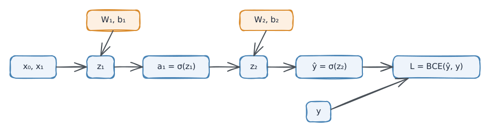
2 hidden neurons: h0 and h1, both using sigmoid activation σ
1 output neuron: y^∈(0,1), the predicted probability of the positive class
Loss: Binary cross-entropy (BCE)
1.1 The Full Network Diagram
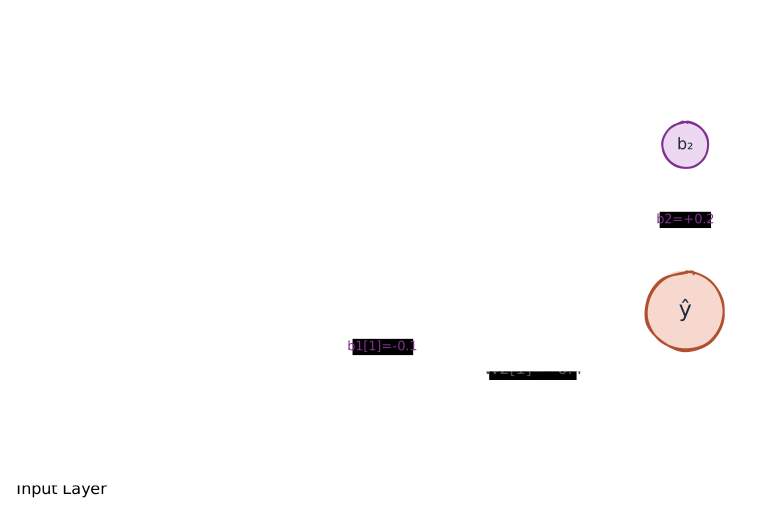
Figure 1: Complete 2-2-1 MLP. Every solid arrow is a learnable weight. Every dashed purple arrow is a bias.
1.2 How to Read the Diagram
Every arrow represents one number: a weight. There are exactly 6 weight arrows and 3 bias arrows. The matrices W1, W2, b1, b2 are just a compact way of writing down all those arrows.
2. What the Weight Matrices Actually Mean
2.1 W1 — Input-to-Hidden Weights
W1 is shape 2×2 because there are 2 hidden neurons (rows) and 2 inputs (columns). The rule is: row = destination, column = source.
W1=row 0 = weights arriving at h0,row 1 = weights arriving at h1(0.50.2−0.30.8)
Entry
Value
Arrow in Figure 1
What it means
W1[0,0]
+0.5
x0→h0
x0 moderately encourages h0 to fire
W1[0,1]
−0.3
x1→h0
x1 suppresses h0; negative weights are inhibitory
W1[1,0]
+0.2
x0→h1
x0 weakly encourages h1
W1[1,1]
+0.8
x1→h1
x1 strongly drives h1
Sign rule: positive weight ⇒ larger input ⇒ neuron fires more. Negative weight ⇒ larger input ⇒ neuron fires less. Magnitude ⇒ strength of the influence.
2.2 b1 — Hidden Layer Biases
b1=(+0.1−0.1)
The bias is an always-on input of 1 multiplied by this stored value. It shifts the neuron's firing threshold independently of any input.
b1[0]=+0.1: h0 gets a small head-start. Even if x0=x1=0, h0's pre-activation starts at +0.1 instead of zero.
b1[1]=−0.1: h1 has a handicap. Inputs must overcome −0.1 before it fires with any conviction.
Without biases, every decision boundary in every neuron would be forced to pass through the origin — a severe restriction on what the network can represent.
2.3 W2 — Hidden-to-Output Weights
Only one output neuron, so W2 has only one row — effectively a flat vector:
W2=(+0.7−0.4)
Entry
Value
Arrow
What it means
W2[0]
+0.7
h0→y^
When h0 fires strongly, y^ increases (votes positive)
W2[1]
−0.4
h1→y^
When h1 fires strongly, y^ decreases (votes negative)
h0 and h1 pull the output in opposite directions. The final prediction is their weighted tug-of-war.
2.4 b2 — Output Bias
b2=+0.2
Single scalar. Before any input is considered, the output pre-activation starts at +0.2, which pushes y^ slightly above 0.5 (towards predicting the positive class by default). Training will adjust this.
2.5 Why We Pick Any Values At All — The Symmetry Problem
We cannot start all weights at zero. If every weight is identical, every neuron in a layer produces the same output, receives the same gradient, and gets the same update — they are stuck in perfect symmetry forever and the network cannot specialise.
We initialise with small random values to break this symmetry. The specific values here are chosen for readability, not realism. In practice, schemes like Xavier or He initialisation are used. But whatever we start with, training will overwrite them.
Purpose: Given the current weights, compute the network's prediction y^ for one input x, then measure how wrong that prediction is using the loss L. No weights change during a forward pass. It is purely a measurement.
We trace Sample 1: x=[1.0,0.5], true label y=1.
4.1 Step 1 — Hidden Pre-Activations z1
Each hidden neuron takes a weighted sum of all inputs plus its bias. This is literally just the dot product of one row of W1 with the input vector, plus the bias.
Why apply a nonlinearity? Without it, stacking two linear layers gives W2(W1x)=(W2W1)x — one big linear layer. No matter how many layers you add, the network can only represent a hyperplane. Sigmoid (or any nonlinearity) makes each layer irreducible — every additional layer genuinely expands what the network can represent.
The network predicts a 59.35% probability for the positive class. The true label is 1. The prediction is wrong-ish — not confident enough in the right direction.
4.5 Step 5 — Loss L
Binary cross-entropy. For y=1, the second term vanishes:
L=−ylogy^−(1−y)log(1−y^)=−log(0.5935)≈0.522
The loss is a single scalar measuring how bad the prediction was. The job of the backward pass is to figure out which weights caused this 0.522 and by how much.
5. The Backward Pass
Purpose: Compute ∂w∂L for every weight w in the network. This gradient tells us the direction in which changing w would increase L. So to decreaseL, we will later move each weight opposite to its gradient.
The backward pass does not change any weights. It only produces gradient numbers.
The mechanism is the chain rule. The loss L depends on y^, which depends on z2, which depends on W2 and a1, which depends on z1, which depends on W1 and x. We unwind this chain in reverse.
Important distinction: the backward pass must calculate gradients for the parameters only: W2[0], W2[1], b2, the four entries of W1, and the two entries of b1. Quantities like z2, a1[0], and z1[0] are not learned, but we still compute derivatives with respect to them as intermediate stepping stones. The "error signals" δ2 and δ1 are exactly these stepping-stone derivatives.
For Sample 1, the scalar computation graph is:
So the full reverse route is:
L→y^→z2→{W2,b2,a1→z1→W1,b1.
The output error signal is not a new assumption. It is a shortcut name for one derivative:
δ2=∂z2∂L.
Once δ2 is known, the output-layer parameter gradients become one-line chain-rule calculations.
We define the error signalδ at each layer:
δ(l)=∂z(l)∂L
This answers: "how urgently does this layer's pre-activation need to change?" It is the central quantity flowing backwards through the network.
5.1 Step 1 — Output Error Signal δ2
For a general binary label y∈{0,1}, the BCE loss is
L=−(ylog(y^)+(1−y)log(1−y^)).
Therefore
∂y^∂L=−y^y+1−y^1−y.
For Sample 1, y=1, so this reduces to ∂L/∂y^=−1/y^.
δ2=∂z2∂L=−1/y^∂y^∂L⋅y^(1−y^)∂z2∂y^
For BCE loss + sigmoid output, these factors cancel exactly:
δ2=y^−y=0.5935−1=−0.4065
If we do not use the shortcut, the Sample 1 calculation is:
∂z2∂L=(−0.59351)(0.5935)(1−0.5935)=−0.4065.
So yes: y^−y is just a compact shortcut for the full chain L→y^→z2.
Interpretation: the negative sign says z2 must increase (the network was too low). The magnitude 0.4065 says how urgently.
This cancellation (y^−y) is one reason BCE + sigmoid is preferred over MSE + sigmoid. With MSE the gradient contains an extra σ′(z2) factor which approaches zero when the network is confidently wrong — learning stalls at exactly the worst moment.
5.2 Step 2 — Gradients for W2 and b2
Since z2=W2[0]⋅a1[0]+W2[1]⋅a1[1]+b2, we have ∂z2/∂W2[i]=a1[i]. By chain rule:
All negative: we should increase all three parameters to reduce the loss. Makes sense — the output was too low (y^=0.594) for a true positive case.
Universal pattern: weight gradient = (downstream error signal) × (the input that weight received). This is always an outer product. Every layer in every architecture follows this.
5.3 Step 3 — Propagate Error Signal Back Through W2
Before we can compute gradients for W1, we need to know how each hidden activation a1[i] contributed to the loss. By chain rule:
h0 needs to increase its output (negative gradient means increasing a1[0] decreases L). h1 needs to decrease its output — because its weight to the output is −0.4, increasing h1 would push y^down, which makes things worse.
5.4 Step 4 — Pass Back Through the Sigmoid
To get the error signal at the hidden pre-activations z1, we multiply by the sigmoid's derivative.
The Vanishing Gradient Problem, live:σ′(z)≤0.25 always — it peaks at 0.25 when z=0. Every sigmoid layer attenuates the error signal by at least 4×.
In our two-layer network: ∣δ2∣=0.4065→∣δ1∣≈0.068. That is already a 6× reduction in one layer. With ten sigmoid layers, δ at layer 1 approaches zero — weights there receive near-zero gradient and stop learning entirely. This is why modern networks use ReLU instead of sigmoid in hidden layers: ReLU′(z)=1 for z>0, so gradient passes through unchanged.
The intermediate derivatives δ2, ∂L/∂a1[0], ∂L/∂a1[1], δ1[0], and δ1[1] are calculated only to make those nine parameter gradients easy to obtain.
6. Gradient Descent: Where Learning Happens
The backward pass measured how each weight contributed to the error. Gradient descent is the step that acts on that measurement. These are two separate steps.
Move each weight a small step opposite to its gradient:
Negative gradient ⇒ increasing w decreases L⇒ move wup
Positive gradient ⇒ increasing w increases L⇒ move wdown
α is the learning rate: the step size. Too large and you overshoot and diverge. Too small and training takes forever. We use α=0.1.
We do not apply this update yet. In mini-batch gradient descent we first average gradients across all samples in a batch, then apply one update. This is explained in the next section.
7. Batches — Aggregating Gradients Before Updating
Why batch? Gradient descent on a single sample is noisy — one unusual sample could point in the wrong direction. Averaging gradients across a batch gives a more stable estimate of which direction actually reduces loss across the data distribution. One weight update per batch, not per sample.
7.1 Forward and Backward Pass for Sample 2: x = [0.2, 0.9], y = 0
Sample 1 says "push W2[0] down." Sample 2 says "push W2[0] up." They partially disagree. The batch average computes the net direction: slightly up (+0.013). With thousands of samples per batch this averaging cancels individual noise and gives a stable, reliable gradient estimate.
7.3 Apply Gradient Descent: One Weight Update
w←w−α⋅gˉ,α=0.1
Parameter
Old value
−α⋅gˉ
New value
W2[0]
+0.7000
−(0.1)(+0.0130)=−0.0013
+0.6987
W2[1]
−0.4000
−(0.1)(+0.0608)=−0.0061
−0.4061
b2
+0.2000
−(0.1)(+0.0808)=−0.0081
+0.1919
W1[0,0]
+0.5000
−(0.1)(−0.0239)=+0.0024
+0.5024
W1[0,1]
−0.3000
−(0.1)(+0.0278)=−0.0028
−0.3028
W1[1,0]
+0.2000
−(0.1)(+0.0140)=−0.0014
+0.1986
W1[1,1]
+0.8000
−(0.1)(−0.0134)=+0.0013
+0.8013
b1[0]
+0.1000
−(0.1)(+0.0158)=−0.0016
+0.0984
b1[1]
−0.1000
−(0.1)(−0.0064)=+0.0006
−0.0994
The changes are tiny. That is expected at step 1 with a cautious learning rate. Over hundreds of epochs these small, consistent nudges accumulate into weights that produce accurate predictions.
8. Epochs — The Full Training Loop
One epoch = one complete pass through every training sample exactly once. With 4 samples and batch size 2: one epoch = 2 batches = 2 weight updates.
8.2 Critical Point: Reset Gradients Across Batches
Within a batch: gradients are averaged across samples, then one update is applied.
Across batches within an epoch: there is no accumulation. Batch 2 runs on whatever weights Batch 1 left behind. The gradients computed in Batch 1 do not directly influence Batch 2 — they influenced the weights that Batch 2 inherits. The effect is indirect, via the updated weight values.
8.3 What the Epoch Loss Number in Training Logs Means
When training prints:
Epoch 1/100 --- loss: 0.680
That 0.680 is the average of all per-sample losses collected during forward passes of that epoch:
Lepoch=N1i=1∑NLi=4L1+L2+L3+L4
This is a monitoring number. It is computed from forward passes. It does not control the weight updates. Its only purpose: tell you whether the model is improving over time. If this number decreases epoch-to-epoch, training is working.
9. Summary: Every Step and Its Role
Step
Changes weights?
Purpose
Forward pass
No
Push input x through the network to produce y^. Compute loss L. This is measurement only.
Backward pass
No
Use the chain rule to compute ∂L/∂w for every weight. Determines how much each weight is "to blame" for the error.
Gradient descent
Yes
Apply w←w−α∇w. This is the only step that actually changes the weights. It is where learning happens.
Batch
—
The set of samples over which gradients are averaged before one weight update. Larger batches give smoother gradients; smaller batches introduce noise that can help escape local minima.
Epoch
—
One complete pass through the full training set. Contains multiple batches. Contains multiple weight updates. The epoch loss is a scalar monitoring metric computed from the forward passes of that epoch.
The complete training loop in pseudocode:
for epoch in 1..num_epochs:
    shuffle(dataset)
    epoch_losses = []

    for batch in chunks(dataset, size=batch_size):

        # Forward pass --- no weight change
        for sample in batch:
            y_hat = forward(sample.x, weights)
            L     = loss(y_hat, sample.y)
            epoch_losses.append(L)

        # Backward pass --- no weight change
        grads = mean([backprop(sample, weights) for sample in batch])

        # Gradient descent --- ONLY step that changes weights
        weights = weights - alpha * grads

    print("Epoch loss:", mean(epoch_losses))   # monitoring only